The headline targets for any U.S. quick-service unit in 2026: ACSI industry CSAT at 79 (with order accuracy sub-score at a benchmark level and beverage quality at a benchmark level), median drive-thru total service time near industry median ranges, and healthy four-wall EBITDA within typical industry margin ranges.
Three immediate actions to run before you finish reading:
- Pull the last seven days of POS data and compare your average unit volume and average ticket against the segment targets in Section 2.
- Run a single timed drive-thru sample or mystery shop during your highest-volume daypart and record total service time from menu-board arrival to food delivery.
- Flag every metric that sits more than 10% outside the targets below and rank them by revenue impact for your first experiment.
Stat to know: The 2025 Drive-Thru Study used roughly 165 mystery shops per brand. AI-enabled locations averaged a total service time notably faster than the study average, improving operational efficiency that compounds across thousands of daily transactions.
Key Takeaways
The most durable quick service benchmarks for U.S.
| Point | Details |
|---|---|
| CSAT and accuracy targets | Industry CSAT sits at 79 (ACSI 2026); order accuracy sub-score is 87 — both are weekly tracking floors. |
| Drive-thru median benchmark | Total service time median is ~330 seconds; AI-enabled pilots averaged 3 minutes 53 seconds, 21 seconds faster. |
| Prime cost discipline | Prime cost (food + labor) must stay below 60%; sustained overage signals a structural margin problem. |
| Four-wall EBITDA range | Healthy units operate at 18–22% four-wall EBITDA; units below 15% require immediate triage. |
| Weekly review cadence | Review food cost, labor %, and prime cost weekly — monthly P&L reviews surface problems too late to act. |
Table of Contents
- What are the core quick service benchmarks every operation should track?
- How do reputation and digital channel benchmarks compare across QSR brands?
- What drive-thru timing benchmarks should you use by daypart?
- What financial benchmarks define a healthy QSR unit?
- How do you build reproducible QSR benchmarks from POS and mystery-shop data?
- How do you prioritize operational improvements when benchmarks show gaps?
- Ready-to-use KPI table template for your dashboard
- Wendy’s AI drive-thru pilots: what moved and what to measure
- How an operations leader should use these benchmarks
- Sources
What are the core quick service benchmarks every operation should track?
The term “quick service benchmarks” covers a specific set of operational and financial KPIs that the industry uses to compare unit performance across formats, dayparts, and ownership structures. Below are the definitions and the industry-average ranges that matter most.
Same-store sales (SSS) growth measures revenue change at units open at least 13 months, stripping out new-unit distortion. A positive SSS trend is the primary signal of brand health; decompose it into traffic change and average check change, because the two require different operational responses.
Average unit volume (AUV) is total annual revenue per location. AUV varies sharply by format: a high-throughput burger chain differs structurally from a sandwich or pizza concept. Use AUV-to-investment ratios rather than raw AUV when comparing across formats.
Average ticket (ATS) represents revenue per transaction. Industry data places a working reference for full-menu QSRs around $12.50, though check inflation since 2022 has pushed many brands above that level.
Transactions per labor hour (TPLH) is the throughput efficiency metric. It connects staffing decisions directly to revenue capacity and is the fastest way to spot over- or understaffing by daypart.
Drive-thru total time covers menu-board arrival to food delivery. The industry median sits near 330 seconds, with top performers consistently below 270 seconds.
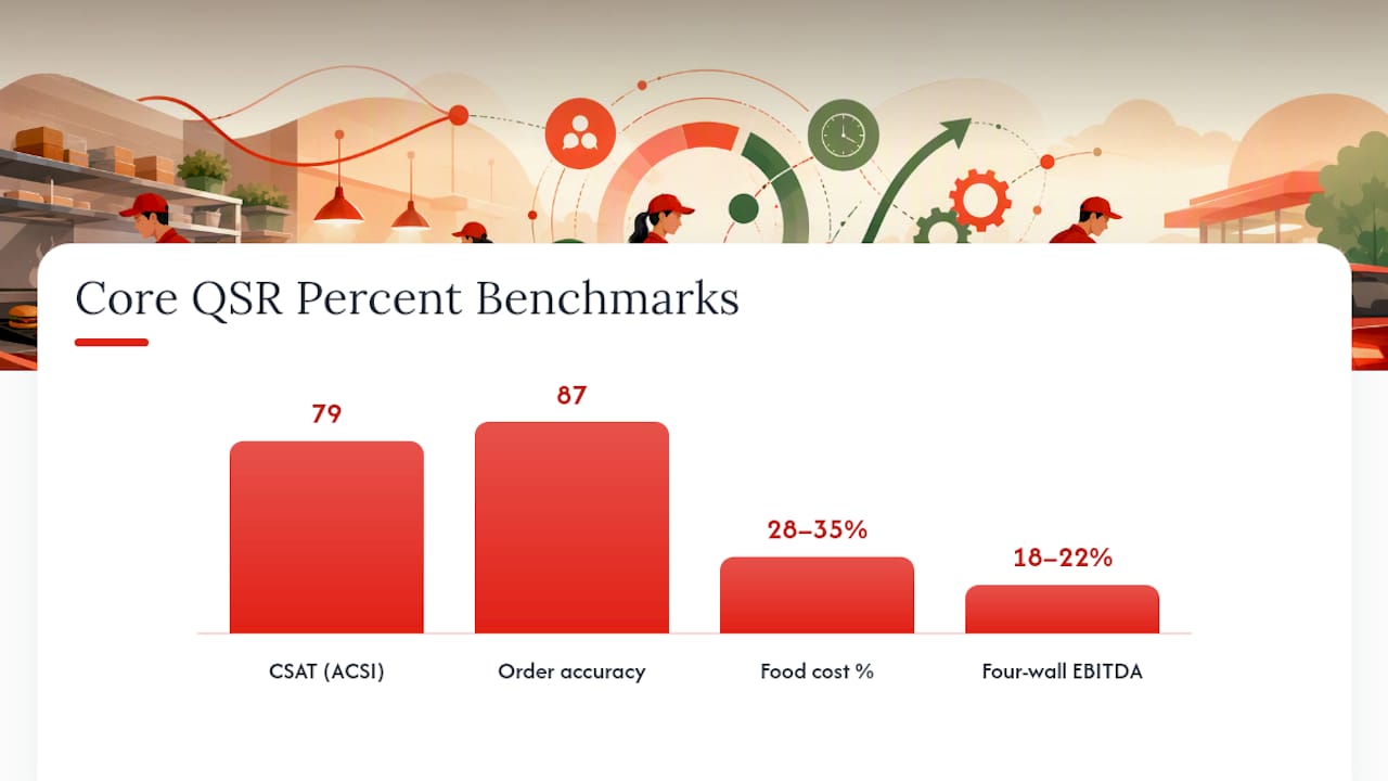
Order accuracy is the percentage of orders delivered correctly on the first attempt. The ACSI sub-score for order accuracy across the quick-service sector is 87 out of 100 for the April 2025–March 2026 period.
CSAT / NPS captures customer satisfaction. ACSI reports the 2026 QSR industry score at 79.
Food cost percentage (CoGS %) is cost of goods sold divided by net sales.
Four-wall EBITDA is the unit-level earnings before interest, taxes, depreciation, and amortization, after all direct operating costs. The PulseRevOps benchmark places a healthy range at 18–22%.
| Metric | Industry average / range | Top / median / bottom variance | Measurement method | Recommended threshold | Cadence |
|---|---|---|---|---|---|
| CSAT (ACSI) | 79 | Top brands: 87; bottom: — | Survey aggregator | ≥79 | Monthly |
| Order accuracy | 87 | Top: 90+; bottom: 87 | Mystery shop / POS | ≥87 | Weekly |
| Drive-thru total time | ~330s | Top: <270s; bottom: >400s | Mystery shop / POS timer | ≤330s | Daily |
| Average ticket | ~$12.50 (reference) | Varies by format | POS extract | Segment-specific | Daily |
| Food cost % | 28–35% | Beverage-heavy: 28–30%; full-menu: 32–35% | POS / inventory | <35% | Weekly |
| Labor % | 25–32% | Lean formats: 25–27%; complex menus: 30–32% | Payroll / POS | <32% | Weekly |
| Prime cost | <60% | Best-in-class: 28–35% | Payroll + COGS | <60% | Weekly |
| Four-wall EBITDA | 18–22% | Top operators: 22–25%; distressed: <15% | P&L | ≥18% | Monthly |
| Same-store sales growth | Varies by macro cycle | Positive traffic + check | POS comps | Positive traffic | Weekly |
For a deeper breakdown of which financial metrics carry the most weight in a QSR profitability model, the QSR profitability metrics guide on Buywendys covers the highest-impact levers in detail.
How do reputation and digital channel benchmarks compare across QSR brands?
Reputation data is increasingly a leading indicator of traffic trends, not a lagging one. A sustained drop in star rating or a spike in review velocity often precedes a measurable decline in transactions by four to six weeks.
Star rating targets: A 4.0 or above on Google Maps is the working floor for a healthy QSR unit. Brands like Chick-fil-A and Raising Cane’s consistently score above 4.2 at the unit level, while brands with service-time or accuracy issues often cluster below 3.8. Five Guys and Jersey Mike’s tend to hold strong ratings on the strength of product quality perception.
Review volume and velocity: Review volume should scale roughly with market share and transaction count. A sudden spike in one-star reviews over a 48-hour window is a stronger signal than the absolute rating, because it often reflects a specific operational failure (a staffing gap, a product quality issue, or a POS outage) rather than a structural problem.
ACSI sub-metrics for 2026: Beyond the headline score of 79, the ACSI data shows order accuracy at 87 and beverage quality at a benchmark level. Brands like Starbucks, Dunkin’, and Panera Bread carry beverage quality as a primary satisfaction driver, making that 85 sub-score particularly relevant for their operators. McDonald’s, Burger King, Popeyes, and KFC compete more on speed and value perception, so their CSAT profiles weight order accuracy and service time more heavily.
Subway, Domino’s, and Starbucks operate well above that floor. Wingstop has publicly cited digital orders as the majority of its sales. For brands like Sonic, Taco Bell, and Pizza Hut, app-based ordering also captures valuable daypart and preference data that third-party marketplaces do not share back to the operator.
First-party vs. third-party split: First-party digital orders (brand app or website) preserve margin and customer data. Third-party marketplace orders carry commission rates that can compress four-wall EBITDA by 3–5 percentage points on affected transactions. Tracking the first-party share of digital sales weekly is a direct proxy for margin health.
Measurement checklist:
- Pull Google Business Profile ratings and review counts weekly for each unit.
- Track review velocity (new reviews per week) and flag units where one-star velocity doubles over a two-week period.
- Monitor app store ratings (iOS and Android) monthly; a drop below 4.0 on either platform correlates with order friction.
- Report loyalty penetration as a share of transactions or sales, not cumulative enrollment totals.
Pro Tip: Cumulative loyalty enrollment figures are a vanity metric. Always measure loyalty as a share of weekly transactions or weekly sales.
What drive-thru timing benchmarks should you use by daypart?
Drive-thru performance is the single most-studied dimension of QSR operations, and the 2025 Drive-Thru Study from InTouch Insight provides the most granular public dataset available, built on approximately 165 mystery shops per brand. The study average for total service time across all brands and dayparts was approximately 4 minutes 15 seconds (255 seconds from order to delivery, with total time including approach and payment closer to 330 seconds depending on measurement convention). AI-enabled drive-thru locations in the pilot sample averaged 3 minutes 53 seconds, roughly 21 seconds faster.
Daypart benchmarks and thresholds:
- Breakfast (6–10 AM): Highest transaction density; service times tend to run 10–15% faster than the daily average due to simplified order complexity. Treat any breakfast daypart averaging above 350 seconds as a staffing or sequencing problem.
- Lunch (11 AM–2 PM): Peak complexity. Order size and customization requests peak here. The industry median for lunch drive-thru runs near 340–360 seconds; top performers hold below 300 seconds.
- Afternoon (2–5 PM): Lower volume but often the slowest per-transaction times due to reduced staffing. Brands like Starbucks and Dunkin’ face disproportionate afternoon pressure from beverage customization.
- Dinner (5–8 PM): Second-highest volume, with family-size orders increasing average ticket and service time. Dinner drive-thru times at full-menu QSRs (McDonald’s, Wendy’s, Burger King, KFC, Popeyes, Taco Bell) typically run 15–20 seconds longer than breakfast.
Stat to know: AI-enabled drive-thru pilots averaged 3 minutes 53 seconds versus the study average of 4 minutes 15 seconds — a 21-second improvement that, at 300 daily drive-thru transactions, translates to roughly 105 minutes of recovered throughput capacity per day.
Order accuracy by format: Accuracy correlates directly with waste and CSAT. Brands with high customization (Subway, Five Guys, Wingstop) face structurally higher accuracy risk than standardized-menu formats. A 1-percentage-point drop in accuracy at a unit doing 500 daily transactions means five incorrect orders per day, each carrying a remade-item cost and a CSAT penalty.
Methodology note: The InTouch Insight study used trained mystery shoppers who recorded timestamps at menu-board arrival, order completion, payment, and food delivery. POS-based timing captures payment-to-delivery but misses the approach and order phases, so POS and mystery-shop data are not directly comparable without a conversion factor. When building internal benchmarks, define your measurement start and end points explicitly and apply them consistently.
What financial benchmarks define a healthy QSR unit?
The cost structure of a QSR unit follows a fairly consistent architecture across formats, though the specific percentages shift with menu complexity, real estate type, and ownership model. IBISWorld’s industry research and the National Restaurant Association’s State of the Industry 2025 report both confirm that cost pressures on labor and food have compressed margins since 2022, making the EBITDA floor harder to hold for operators without scale or pricing power.
The workable ranges for a U.S. QSR unit:
- Food cost (CoGS %): 28–35%. Beverage-focused formats (Starbucks, Dunkin’) run toward the low end; protein-heavy menus (Five Guys, Raising Cane’s, Popeyes) run toward the high end. A food cost above 35% on a sustained basis signals portion-control drift, waste, or supplier pricing that needs renegotiation.
- Labor %: 25–32% of net sales. This range has widened since 2022 as minimum wage increases took effect in California, New York, and other high-cost states. Brands with high drive-thru throughput (Chick-fil-A, McDonald’s) tend to hold labor closer to 27–28% through volume leverage.
- Prime cost (food + labor): Target below 60%. Prime cost above 62% leaves less than 38% of revenue to cover occupancy, utilities, royalties, and profit, which is structurally insufficient for most franchise models.
- Occupancy (rent + CAM): Typically 8–10% of net sales for a well-sited unit. End-cap and freestanding drive-thru formats tend to carry higher absolute rent but benefit from higher AUV, keeping the percentage manageable.
- Four-wall EBITDA: 18–22% is the healthy range. Units below 15% are typically in distress or in a ramp-up phase. Units above 22% are either exceptionally well-run or operating in a low-cost market.
For AUV context: high-volume burger and chicken formats (McDonald’s, Chick-fil-A) operate at materially higher AUVs than sandwich or pizza concepts (Subway, Jersey Mike’s, Pizza Hut). The AUV-to-investment ratio matters more than raw AUV when evaluating franchisee returns, because a $2.5M AUV unit that required $1.8M to build is structurally different from a $1.5M AUV unit built for $400K.
Weekly financial review snapshot (recommended fields):
- Net sales vs. prior week and prior year (same week)
- Food cost % (actual vs. target)
- Labor % (actual vs. target, broken out by daypart)
- Prime cost (combined)
- Average ticket and transaction count
- Any promotional period flags that affect CoGS comparability
NetSuite’s restaurant benchmarking guidance recommends reviewing COGS, labor, and profitability at least weekly to catch unit-economics gaps before they compound. A monthly review cadence is too slow for food cost and labor; by the time a monthly P&L surfaces a problem, four weeks of margin erosion have already occurred.
For a detailed breakdown of how restaurant operating margins compare across QSR formats, Buywendys maintains a dedicated reference page with current ranges.
How do you build reproducible QSR benchmarks from POS and mystery-shop data?
Reproducibility is what separates a defensible benchmark from an anecdote. The methodology below reflects the approach used in the InTouch Insight drive-thru study and adapted for internal portfolio use.
Data sources and when to use each:
- POS extracts: Best for financial KPIs (AUV, ATS, food cost, labor), transaction counts, and daypart throughput. Limitations: POS captures payment-to-delivery timing but not approach or order phases; it also reflects net sales after voids and comps, which can distort food cost if not reconciled.
- Mystery shops: Best for service-time components, order accuracy, and customer experience quality. The InTouch Insight standard of roughly 165 shops per brand provides statistical reliability at the brand level; for a single-unit operator, 20–30 shops per quarter per daypart is a workable minimum.
- App telemetry and review aggregators: Best for digital channel mix, loyalty penetration, and reputation velocity. Pull weekly; do not rely on monthly snapshots for reputation data.
- Third-party industry reports (ACSI, IBISWorld, InTouch Insight): Best for external calibration. Use these to set the benchmark targets your internal data is measured against.
Sample size guidelines:
- For a drive-thru timing study equivalent to the InTouch Insight methodology, target 165 mystery shops per brand or concept, spread across all dayparts and at least three geographic market types (urban, suburban, rural).
- For a single-unit POS baseline, use a minimum of 28 consecutive days, excluding any promotional launch weeks that would distort the baseline.
- For daypart analysis, ensure each daypart (breakfast, lunch, afternoon, dinner) has at least 20 data points before drawing conclusions.
Normalization rules:
- Adjust for market-size weighting when aggregating across a portfolio with units in both high-cost metros and lower-cost markets. A labor % of 30% in San Francisco and 30% in rural Ohio represent very different operational realities.
- Strip promotional periods from CoGS benchmarks, or flag them explicitly. Value deals and product refreshes materially move comps in the short term; Q2 2026 business reporting shows how promotional programs at brands like Burger King influenced short-term comp results in ways that would distort a clean benchmark comparison.
- Separate company-operated and franchised units when benchmarking EBITDA, because royalty and rent structures differ.
- Adjust for check inflation when comparing ATS across years. A $13.50 average ticket in 2026 is not directly comparable to a $10.50 ticket in 2022 without a menu-price deflator.
Methodology checklist:
- Define measurement start and end points for every timing metric before collecting data.
- Document the data source (POS, mystery shop, aggregator) and the collection period for every KPI.
- Flag and exclude promotional weeks from baseline calculations.
- Apply market-size and daypart-mix weights before aggregating across units.
- Validate internal benchmarks against at least one external reference (ACSI, InTouch Insight, IBISWorld) annually.
How do you prioritize operational improvements when benchmarks show gaps?
Not every benchmark gap deserves the same response. The prioritization framework below helps operations leaders allocate attention and experiment budget.
Impact vs. ease matrix:
| Gap type | Revenue / margin impact | Ease of fix | Priority |
|---|---|---|---|
| Drive-thru time >350s at lunch | High (throughput capacity) | Medium (staffing reallocation) | 1 |
| Food cost >35% sustained | High (direct margin) | Medium (portion control, supplier) | 1 |
| Order accuracy <85% | High (waste + CSAT) | Medium (training, line check) | 1 |
| Labor % >32% | High (margin) | Low (scheduling, volume needed) | 2 |
| CSAT below industry score | Medium (traffic trend) | Low (multi-factor) | 2 |
| Average ticket below segment | Medium (revenue) | Medium (suggestive selling, menu) | 2 |
| Review velocity spike | Low immediate, high if sustained | High (respond + investigate) | 3 |
Experiment template for each priority gap:
- Hypothesis: State the specific change and the expected directional effect (e.g., “Adding a dedicated order-taker at the speaker during lunch will reduce total service time by at least 20 seconds”).
- Metric to track: One primary metric (total service time) and one secondary metric (labor % for that daypart).
- Sample size and duration: Minimum 14 days, minimum 20 mystery shops or 200 POS transactions per daypart.
- Success criteria: Define the threshold before the experiment starts (e.g., median service time below 310 seconds with no increase in labor % above 29%).
- Owner: Assign a single named person responsible for data collection and weekly reporting.
Concrete plays by gap type:
- Food cost high: Run a 30-day portion-control audit using weighed portions against recipe standards. Track CoGS weekly. A 1-percentage-point reduction in food cost at a $1.5M AUV unit saves $15K annually.
- Drive-thru slow: Test speaker-clarity improvements and staffing reallocation to a dedicated order-taker position during the problem daypart. Measure before and after with mystery shops.
- Order accuracy low: Implement a line-check protocol at the bagging station and track accuracy via mystery shop weekly for 30 days.
- Average ticket below target: Test a structured suggestive-selling prompt at the speaker or POS screen. Measure ATS change over 21 days against a control group of units.
Ready-to-use KPI table template for your dashboard
The fields below represent a complete weekly snapshot template. Populate each row from POS extracts and mystery-shop data using the definitions in Section 2.
How to populate this template from POS and mystery-shop data:
- Export daily POS transaction files and calculate ATS and food cost % at the unit level before aggregating.
- Enter mystery-shop results within 48 hours of the shop date to keep timing data current.
- Flag any week that includes a promotional launch or LTO introduction with a “promo week” tag so it can be excluded from baseline calculations.
- Review prime cost weekly; if it exceeds 60%, identify whether the driver is food cost or labor before taking action.
CSV field formatting rules for dashboard import:
- Date field: YYYY-MM-DD
- Numeric fields: two decimal places, no currency symbols in data cells
- Daypart field: use standardized labels (Breakfast, Lunch, Afternoon, Dinner) with consistent capitalization
- Source field: POS, Mystery Shop, Survey, Calculated
- Promo flag: Boolean (Y/N)
Wendy’s AI drive-thru pilots: what moved and what to measure
Wendy’s FreshAI deployment represents the most publicly documented AI drive-thru pilot in the U.S. QSR sector, making it the most useful case study for practitioners evaluating whether voice AI belongs in their own benchmarking framework. The 2025 Drive-Thru Study captured AI-enabled locations averaging 3 minutes 53 seconds total service time versus the study average of 4 minutes 15 seconds, a 21-second improvement in the sampled pilot sites.
What the pilot changed operationally:
- Voice AI handled initial order-taking at the speaker, reducing the cognitive load on crew during peak periods.
- Suggestive selling prompts were delivered consistently on every transaction, which human order-takers execute inconsistently under volume pressure.
- Speaker clarity improved in pilot locations, reducing order repetition and the associated time cost.
What the data does not yet confirm: The pilot sample is not large enough to establish statistical significance across all dayparts and market types. Breakfast and lunch dayparts showed the clearest time improvements; afternoon and dinner results were more variable. Speaker-clarity confounds (background noise, accent recognition gaps) remain a documented limitation.
For a detailed analysis of how FreshAI affects Wendy’s unit economics and investor case, Buywendys covers the AI drive-thru revenue impact in a dedicated analysis.
Implementation checklist for an AI drive-thru pilot:
- Define a minimum of 10 pilot sites and 10 matched control sites before launch.
- Establish a 60-day pre-pilot baseline for service time, order accuracy, and ATS at all sites.
- Measure for a minimum of 90 days post-launch to capture daypart and seasonal variation.
- Collect mystery-shop data at both pilot and control sites using the same timing methodology.
- Set explicit quality gates: if accuracy drops below 85% at any pilot site, pause and investigate before expanding.
Red flags that invalidate pilot results:
- Pilot sites were selected because they were already high-performing (selection bias).
- Measurement methodology changed between baseline and pilot periods.
- A promotional campaign ran during the pilot period, inflating ATS and distorting accuracy comparisons.
- Sample size fell below 20 mystery shops per site per daypart.
Pro Tip: When presenting AI pilot results to franchisees or investors, always report the control-site performance alongside the pilot-site performance. A pilot that shows 21 seconds of improvement means nothing if the control sites improved by 18 seconds over the same period due to seasonal factors.
How an operations leader should use these benchmarks
The most common failure mode in QSR benchmarking is not a lack of data. It is a lack of triage discipline. Operations leaders who track 40 metrics weekly end up acting on none of them with enough precision to move the needle.
The practical deployment of this playbook looks like this: nightly, review transaction count and average ticket against the prior-week equivalent. Monthly, review CSAT, drive-thru timing trends, and digital mix against the industry benchmarks in Section 2.
In the first 30 days with a new portfolio or a newly acquired unit, three actions take priority. First, pull a 28-day POS baseline and map every financial KPI against the ranges in Section 5. Second, run a timed drive-thru sample across all three major dayparts and compare against the 330-second median. Third, reconcile food cost against recipe standards to identify whether overage is a purchasing problem, a portion-control problem, or a waste problem — because each requires a different fix.
When communicating benchmark findings to franchisees, lead with the gap in dollar terms, not percentage terms. A franchisee who hears “your food cost is 2 points high” may not act. A franchisee who hears “that 2-point food cost gap costs your unit approximately $30,000 annually at your current AUV” will schedule a meeting. For investor audiences, the same translation applies: operational benchmark gaps are the leading indicators of the EBITDA compression that shows up in quarterly results six to twelve months later. The fast food industry stock trends analysis on Buywendys connects these operational signals to market-level implications.
Placer.ai’s Q2 2026 data showing a roughly 3.0% year-over-year decline in QSR visits is a reminder that macro headwinds can shift benchmarks in ways that are not unit-specific. When industry-wide traffic falls, a unit holding flat transactions is actually outperforming the benchmark, even though the absolute number looks stagnant. Adjust your interpretation of SSS and transaction benchmarks accordingly during periods of macro-driven traffic pressure.
Sources
The sources below represent the highest-value public references for QSR benchmarking in the U.S. market. Each entry notes what the source covers and why it merits inclusion in a practitioner’s reference set.
- Quick-Service Restaurants | The American Customer Satisfaction Index
- Drive-Thru Study Report 2025 (InTouch Insight)
- What are the key sales KPIs for the Quick Service Restaurant… (PulseRevOps)
- Restaurant benchmarks (NetSuite resource article)
- Fast Food Restaurants industry report (IBISWorld)